Mixture Of Gaussian Model Answer

Mixture Of Gaussian Model

Looking for top-notch assignment services in the UK? Look no further than Native Assignment Help. With our dedicated team of experts, we offer comprehensive assistance tailored to your academic needs, ensuring excellence in every assignment.

Introduction: Mixture Of Gaussians Model

The Gaussian model's graph is parabolic type in nature at the initial stage, where the slope is zero and it climbs up at the centre point and becomes zero after some time. A mixture of the Gaussian model is useful for data mining, recognition pattern machine learning and statistical analysis and many more purposes. For the following features, the Gaussian model becomes an important part of the work and without this the analysis of the different datagram’s becomes difficult. The Gaussian model is very important for prediction-related statistical approaches such as height scores, IQ, sum, age and many more things from the resource data or the data frames.

Background

The Gaussian model helps to analyze different datasets for statistical works means it helps to understand and predict different requirements such as age, height and many more things. For this, the model is popular from the previous time when humans were accustomed to doing mathematical calculations through manual processes or methods; nowadays users are implementing this for such work using python language software work. This is the era of machine learning and in this process identification of the different objects is an important part of the work for this Gaussian model is very helpful and users are using it for this purpose. Data mining is the process of sorting data from large datasets to identify the patterns of the data and for this work, the Gaussian model is helpful because it can fulfil the following purpose in a very short time (Li et al. 2018).

Questions

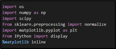
Figure 1: Library importing

To start any analysis or work with such a function it becomes important to import the library and declare the form before. Because this helps the work as per the requirement; in this work, the first command is used to import the so for the work in python. The next command is numpy library importing, this is an important library function and it is very helpful for completing mathematical operations, random number generating and many more mathematical works; this is declared as np here to make coding easier. Scipy is the next library function used for scientific computing and technical computing and it is imported here to make computing easier. Matplotlib is a comprehensive library function used to generate static, iterative animated visualisations in python and for this feature; the following library is used in this work. After declaring the following library functions in GoogleCollab the work is completed targeting to answer some of the questions as per the requirements; the questions and answers are written below.

Question 1

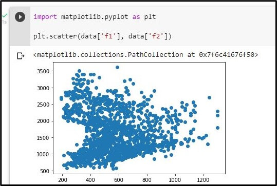
Figure 2: Scatter plot

The following diagram shows the scatter plot of the two data frames f1 and f2, scatter plot is a graphical representation of the data frames to show the values or data distribution and represent null values and corrupted values before removing. In this diagram F1 and F2 are represented along two different axes and the data representing blue dots are in more numbers at the initial position.

Question 2

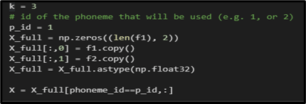
Figure 3: for k=3 the models coding

In this diagram, the coding for the model for the k=3 is represented where k is considered as 3 and to set the id of the phoneme P_id is considered as 1. X_full is defined as an array which may have the values of zero; the array is constructed using the data frame f1.

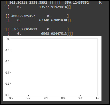
Figure 4: for k=3 the output graph

This diagram shows the graph for the different axis data comparison and to draw the graph the calculator is taken as k=3; this returns the following patterns of the graph (Li et al. 2018).

Question 3

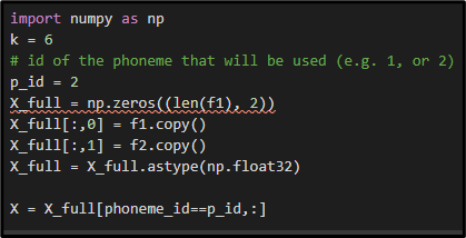
Figure 5: for k=6 and phonemes value=2 the models coding

To complete this requirement the work is done using the numpy library function and k is considered as k=6. Id for the is taken as two. X_full is considered an array which may have the zero value from the f1 data frame. The work is also completed using another three different commands all this thing is represented in the following diagram.

Question 4

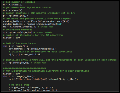
Figure 6: for k=6 repeat training

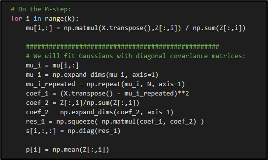
Figure 7: for k=6 repeat training

The following figures show the coding for k=6, phoneme_Id=1 and phoneme_ID=2. To complete this work at first the number of samples for the work is determined using the code and this portion is mentioned in the code using the comment line inside the software. Thereafter the dimension of the data frame is calculated and primary weight gmm weights are taken as 1/k where gmm means the randomly taken data from the samples of the data. Thereafter a covariance matrix is created and the number of iterations is declared as 100 here. Thereafter covariance is initialised and for fractions of the data initial covariance is taken. Thereafter the z array is created to set the value for the Gaussian model in each of the iterations. The expectations maximisation algorithm is written in the next block of the code. In this work for the k=6 value, the Gaussian model is implemented and the whole process is represented using the two diagrams.

Question 5

The following figure shows the process used for the 2Mog when k=3 and this is used to classify between phonemes 1 and phonemes 2. Here at first Inds_1 is represented using a where condition and the inds_2 are defined by the where condition. After some other steps are done in the last two arrays x and n are created using the shape zero and shape one command. Thereafter two phonemes are calculated using the required commands and logical instructions (Das et al. 2019). All the following things are represented using the following diagram.

The following figure depicts the repeat training programme for the Gaussian Model of the k =6. In this work to generate the plot the declaration for the numbers of the samples with mentioning the scale range is done. The scatter plot for the phoneme 1 and for the phoneme 2 is prepared. The phoneme 1 is considered to be plot in colour red and the phoneme 2 is considered to be in the colour of green.

Question 6

This figure shows the information for k =6 and in this work, inds_1 is defined by a where statement where the phoneme value is equal to the one. Similarly, Inds_2 is defined by another where statement where the phoneme_id value is equal to two. In this work the Inds_1 is considered as an array which may have the value of zero and Inds_2 is considered also the same type of array. In the next step, Inds_1 and Inds_2 are merged using the concatenation command in the software and the whole data is set inside a different data frame as the same data types. Thereafter the shape of the x data frame and N data frame is calculated; in the next block of the code, the prediction for different phonemes is represented for the required value of k (Viroliet al. 2019). 

This is the MoG training programme generated for plotting the scatter plot of the phoneme 1 and phoneme2. In this work the phoneme 2 is considered by the red colour and the phoneme 1 is considered by the yellow colour. From this diagram it can be easily said that the amount of the phoneme 2 is higher than phoneme 1 here.

Question 7

The following figure shows the classification diagram for phoneme one and phoneme 2 where phoneme one is represented using the red dots in the figure and phoneme two is represented using the green dots. From the diagram, it is clear that the amount of phoneme one and phoneme two is nearly the same though phoneme two is large in amount (Bandiet al.  2019).

To perform this operation the shape of the data frame N and the data frame D is calculated. In the next step, the minimum value of the f1 data frame and minimum value of the f2 data frame is determined along with their maximum value (Shahinet al. 2019). The maximum of the f1 and minimum of the f1 data frame values difference is assigned inside an N_f1 variable (Zuoet al. 2018). Thereafter the minimum of the f2 and maximum of the f2 data frame values is assigned inside the N_f2 variable. Thereafter two different print statements are used to print the required statements in this work. Thereafter the axis of the figures is defined by the code of the subplot type. In this work, the x-axis is considered as label f1 and the y-axis is considered as label f2. The limits of both axes are set by the minimum value from zero to N_f1 and zero to N_f2 value. Thereafter another set of lines was written to perform the title adding and ranges along with the ticks on the different axes (Koppenet al. 2018).

Question 8.

The following figure shows the output diagram for the following requirements; in this output diagram, the three different axes along with their ranges are represented and to complete or achieve this output diagram the system has computed 150 numbers of the iteration in a few seconds (García-Fernándezet al. 2019).

The following figure shows the required coding for the work, at first matplotlib library function is imported for the work and P_id is considered as 1 n and k = 3. X is defined by an array which may have zero values and the array is constructed using an f1 data frame. In this calculation, the number of the iteration is declared as 150. The initialization of covariance is created in the next steps for the mentioned range of the I. Here the covariance matrix is created as the transpose of the x matrix (Singhal et al. 2020).

The mixture of the Gaussians Model (MOG) is used for the probability distribution of the different dimensional vectors; the commonly used dimensional vectors are of the D dimensional vector. The solution has been made for the problem statement of k=3 and to complete the work at first the importing of the library function is done in the software. After declaring required variables and inserting the values into the variables two loop for completing different iteration is done. The axis and the diagram variables are mentioned inside the scripting portion so that the output is clearly understandable. The fist loop has been prepared to complete the required number of the steps and the second loop function has been used to show the numbers of the iterations for the work. Inside the first loop the operation for the covariance matrix has been performed. Inside the operation portion the transpose of the covariance matrix has been performed.

In this figure the coding for printing the numbers of the iteration for the different steps has been performed and the scripting has been prepared up to the hundred of fifty number of the iteration; all this work has been mentioned inside the appendix portion of this work.

Question 9

The following figure shows the required coding for the work, at first matplotlib library function is imported for the work and P_id is considered as 1 n and k = 6. X is defined by an array which may have zero values and the array is constructed using an f1 data frame. In this calculation, the number of the iteration is declared as 150. The initialization of covariance is created in the next steps for the mentioned range of the I (Li et al. 2020). Here the covariance matrix is created as the transpose of the x matrix. In this diagram, the command fig is used to convert plot values into the figure. The command ax1 is used using a 3d projection command so that the visualisation of the output is generated in a three-dimensional value. The next command line is used to add the required strings in the title portion of the output diagram. In the next stage shape of the x is considered as the value for N and D.Thereafter few more lines of the code are also written after that inside of the for a statement of I variables in the data range of the k the covariance matrix is set up using the required conditions and s for the covariance matrix is also set up. Thereafter the codes for the z variable are also represented to fulfil the requirements. In the next step, a conditional statement is written for the variable t in the range up to the value of the variable n_iter. Inside this conditional statement, a print statement is used to show the numbers of the iterations executed in this operation process. Thereafter inside the conditional statement mu_i is assigned by a value from another variable. Then this value is projected by axis 1 in the graph. Thereafter a repeated variable for the process is created so that this process can be repeated for different iterations and all this thing is projected inside the graphical output (Yuan et al.  2020).

In this work for the following requirements the k=6 are considered as per the requirements from the work. To complete this work the variables has been declared at the first. The functions to of the axis of the plot have been taken so that user can easily understand the graph. The fist loop has been prepared to complete the required number of the steps and the second loop function has been used to show the numbers of the iterations for the work. Inside the first loop the operation for the covariance matrix has been performed. Inside the operation portion the transpose of the covariance matrix has been performed. The plot function has been used in the last parts of the coding to show the plotted output. In this work the print function for printing numbers of the iteration is limited to hundred and fifty lines.

Conclusion

In this work the output diagram of the mixed Gaussians model is created for different values of the k and phonemes values. The total work is completed for different problem questions and the whole result is shown by the different by different output diagrams and the required codes. To complete this work the library importing for different cases in python language is also done as this is an important part of the work.

References

Bandi, H., Bertsimas, D. and Mazumder, R., 2019. Learning a mixture of gaussians via mixed-integer optimization. INFORMS Journal on Optimization, 1(3), pp.221-240.

Das, A., Acharya, U.R., Panda, S.S. and Sabut, S., 2019. Deep learning based liver cancer detection using watershed transform and Gaussian mixture model techniques. Cognitive Systems Research, 54, pp.165-175.

García-Fernández, Á.F., Xia, Y., Granström, K., Svensson, L. and Williams, J.L., 2019, July. Gaussian implementation of the multi-Bernoulli mixture filter. In 2019 22th International Conference on Information Fusion (FUSION) (pp. 1-8). IEEE.

Koppen, P., Feng, Z.H., Kittler, J., Awais, M., Christmas, W., Wu, X.J. and Yin, H.F., 2018. Gaussian mixture 3D morphable face model. Pattern Recognition, 74, pp.617-628.

Li, K., Ma, Z., Robinson, D. and Ma, J., 2018. Identification of typical building daily electricity usage profiles using Gaussian mixture model-based clustering and hierarchical clustering. Applied energy, 231, pp.331-342.

Li, L., Li, W., Du, Q. and Tao, R., 2020. Low-rank and sparse decomposition with mixture of Gaussian for hyperspectral anomaly detection. IEEE Transactions on Cybernetics, 51(9), pp.4363-4372.

Li, Y., Zhang, J., Ma, Z. and Zhang, Y., 2018. Clustering analysis in the wireless propagation channel with a variational Gaussian mixture model. IEEE Transactions on Big Data, 6(2), pp.223-232.

Shahin, I., Nassif, A.B. and Hamsa, S., 2019. Emotion recognition using hybrid Gaussian mixture model and deep neural network. IEEE access, 7, pp.26777-26787.

Singhal, A., Singh, P., Lall, B. and Joshi, S.D., 2020. Modelling and prediction of COVID-19 pandemic using Gaussian mixture model. Chaos, Solitons & Fractals, 138, p.110023.

Viroli, C. and McLachlan, G.J., 2019. Deep Gaussian mixture models. Statistics and Computing, 29(1), pp.43-51.

Yuan, W., Eckart, B., Kim, K., Jampani, V., Fox, D. and Kautz, J., 2020, August. Deepgmr: Learning latent gaussian mixture models for registration. In European conference on computer vision (pp. 733-750). Springer, Cham.

Zuo, H., Lu, J., Zhang, G. and Liu, F., 2018. Fuzzy transfer learning using an infinite gaussian mixture model and active learning. IEEE Transactions on Fuzzy Systems, 27(2), pp.291-303.