Statistics And Data Presentation Coursework Question and Answers

Scenario 1: Fiber Intake in Older Adults

Question 1

An Independent t-test is the appropriate statistical test to analyze this data.

Question 2

Figure 1: Independent sample t-test

The independent sample t-test is a very helpful statistical approach to the hypothesis testing of the research, it helps to determine the fiber intake in older adults, and whether there is a statistical difference between two groups that are living in the community and those adults living in the sheltered or residential accommodations.

This test helps to decrease the demand characteristics. Specifically, the research data consists of continuous variables here the research data is based on the daily intake of fiber in older adults (Makowski, et al 2020).

Finding it hard to express ideas clearly? Our Assignment Writing Help enhances your writing voice and ensures clarity. Let your thoughts flow effortlessly—get a quote today!

This test assumes the data that is distributed normally and it varies in both groups ( the adult who lives in the community and the adult who lives in residential accommodation). Here this test helps to confirm the parametric assumption of the research. Generally, this test is utilized to handle some deviation from the normality test of the variables and the homogeneity test of the different variances.

In this case, the independent variables help to recognize the hypotheses of the research which investigates whether older adults in sheltered or residential housing intake more dietary fiber than those living in their own homes. This test helps to differentiate 2 groups easily as per their intake of dietary fiber.

Question 3

Bar chart

Question 4

Summary data

Question 5

Average daily fiber intake (g/day) of adults living in the community

Question 6

Average daily fiber intake (g/day) of adults living in sheltered or residential accommodation.

Question 7

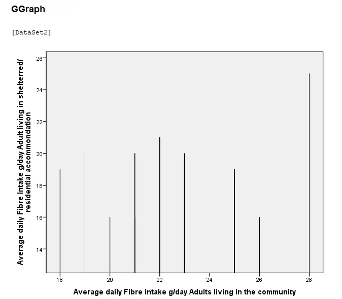
Figure 2: Bar graph

The upper figure demonstrates the graph of the individual people who live in the community and residential accommodation and their differences in consumption of daily dietary intake (Pour‐Aboughadareh, et al.2019). The X-axis defines the people who live in the community and the Y-axis demonstrates the people who live in the residential or sheltered accommodation.

Question 8

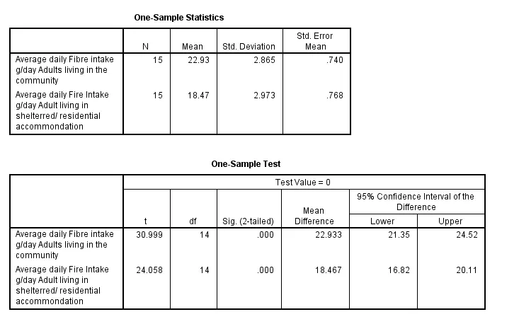
Figure 3: Independent T-test

The upper figure describes the independent T-test of 2 groups of people, one who lives in the community and another who lives in the residential or sheltered accommodation. It helps to demonstrate these two groups of individual people’s dietary fiber intake. For conducting this analysis a total of 30 participants were taken. Among those 30 individuals, 15 candidates are separated who lived in the community and 15 candidates are separated who lived in residential or sheltered accommodation (DeBono, 2021). For the people who live in the community, the mean value of their daily dietary fiber intake is 22.93 and their “standard deviation” is 2.865. For the people who live in sheltered or residential accommodation, the mean value of their daily dietary fiber intake is 18.47 and their “standard deviation” is 2.973.

The t value of the average daily fiber intake for adults who live in the community is 30.999 and the value of df is 14. The mean difference is 22.933. For the people who live in the sheltered and residential accommodation, their t value is 24.058 and the value of df is 14. The mean difference is 18.467.

From the upper result, it has been demonstrated that those people who live in the community their consumption of fiber is higher than the person who live in sheltered or residential accommodations.

Scenario 2: A novel anti-tumor agent

Question 9

Group	Treatment	Number of Mice (Initial)	Number of Mice (End)	Number of Mice with Colon Tumors
Control	Saline	65	65	32
Test	100mg Cumane + Saline	65	65	38

Table 1: A novel anti-tumor agent accuracy testing

The chi-square test is the most appropriate statistical test to analyze this data.

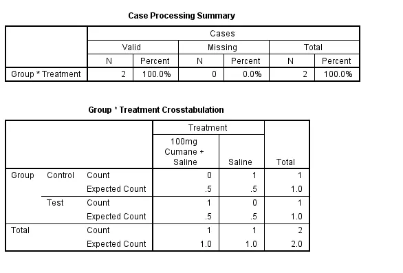
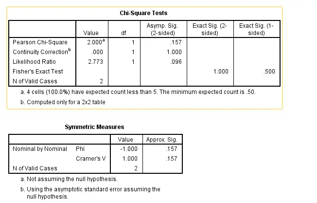
Figure 4: Chi-Square test

Question 10

The chi-square test helps to determine the significant association or difference between the mice that are taken for the research to determine the colon tumors, Here taken anti-cancer agent (cumane) in preventing colon tumors in the control group of mice and the test groups of mice (Turhan, 2020). This is most commonly used by the researchers to determine the effectiveness of the medicines. This is very easy to compute the result of the test. This helps to categorial variables that are interrelated to each other.

Question 11

Bar chart

Question 12

Summary data

Question 13

The X-axis demonstrates the Number of mice taken for the research.

Question 14

The Y-axis demonstrates the number of mice with colon tumors.

Question 15

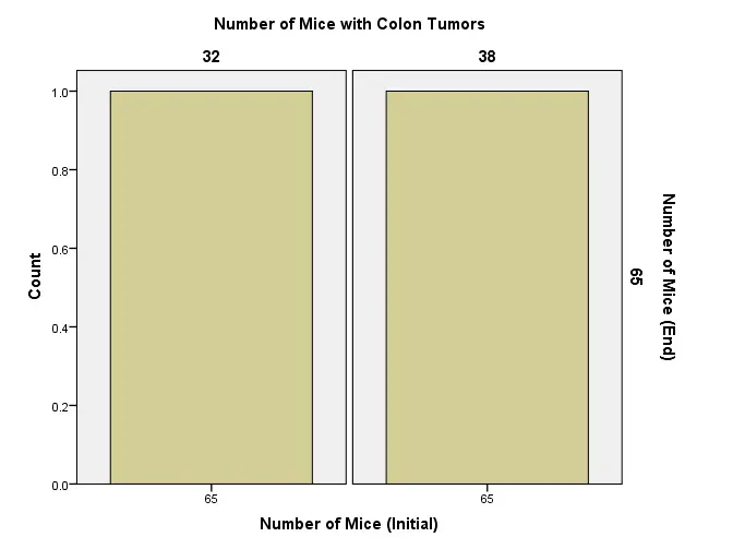
Figure 5: Number of mice with colon tumors

The upper figure demonstrates the bar graph. In the graph, the discussion will be about the accuracy of an anti-cancer agent that is isolated from spinach. It has been noticed that initially 65 mice were taken for this research study (Amin, 2021). The number of mice with colon tumors is 32. At the end of the research study 32 mice in the control group had confirmed colon tumours, whilst in the mice treated with cumane, 38 had tumours.

Question 16

The picture shows a table with the findings from a chi-square independence test. The purpose of the test is to ascertain if two category variables significantly correlate with one another. The table displays the degrees of freedom, p-value, chi-square figures, and predicted and witnessed counts for every cell in the distribution table.

The table displays two different variables, each with two levels. With one unit of liberation, the coefficient of chi-square is 2.773. The statistically relevant criterion of 0.05 is surpassed given a p-value of 0.096. The null explanation, which states that both factors are independent, is unable to be disproved as a consequence.

In general, the graphic indicates a weak but significant statistical relationship among the two parameters.

Scenario 3: Diet and iron status

Question 17

To analyze the data in scenario 3, the one-way ANOVA test is needed.

Question 18

In this part, the one-way ANOVA test is presented for understanding the data properly. Here are some considerations of why among many types of tests the one-way Anova test is taken, is divided one by one point.

1. Number of groups: Three groups—Groups A, B, and C—convey various dietary interventions and are included in the study (Ferreira, 2019). ANOVA is acceptable in this situation because it is made to liken means across many groups.
2. Continuous Dependent Variable: Serum ferritin levels are a persistent, numerical dependent variable that may be used in an ANOVA. The purpose of an ANOVA is to evaluate mean differences for continuous variables.
3. Corresponding Numerous Treatments: The study aims to evaluate the effects on iron status of two distinct dietary treatments (oranges and tea). Numerous groups can be compared simultaneously using an ANOVA to see whether there are any statistically important differences between them.
4. Testing Hypotheses: The objective is to determine if citrus fruits enhance iron status and if the phenolic in tea lowers serum ferritin. ANOVA is a method for evaluating hypotheses that might offer statistical proof of group differences.
5. Deductions: Equivalent variances across groups, normally distributed data, and independence of observations across groups are all considered by one-way ANOVA. To guarantee that the results are legitimate, these presumptions can be verified or rectified as necessary.
6. Post-Hoc Testing: If the ANOVA reveals noteworthy group differences, post hoc analyses can be employed to identify the particular groups that vary from one another, offering a more in-depth understanding of the impacts of the dietary treatments (Carrasco, et al. 2020).

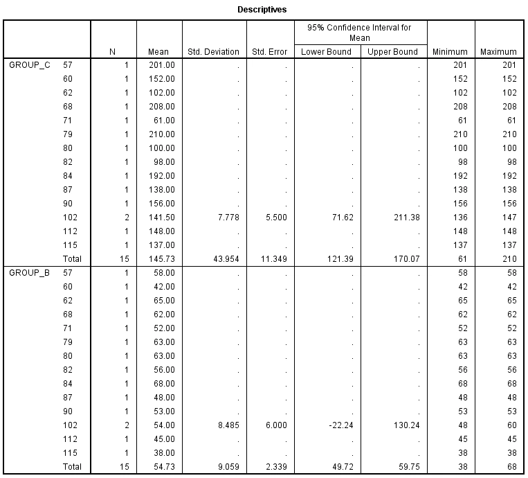
Figure 6: One-way ANOVA test

In conclusion, because of its suitability for handling numerous groups, constant dependent variables, and applicability to evaluating hypotheses about the effects of dietary interventions on iron status, the one-way ANOVA is the statistical test that is most suited for this situation.

Question 19

A bar chart is chosen for presenting the data from scenario 3.

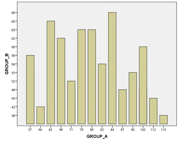
Figure 7: Bar chart

Question 20

Here summary data is chosen to present the data.

Question 21

“Group A” is chosen as the level for the X-axis of the bar graph.

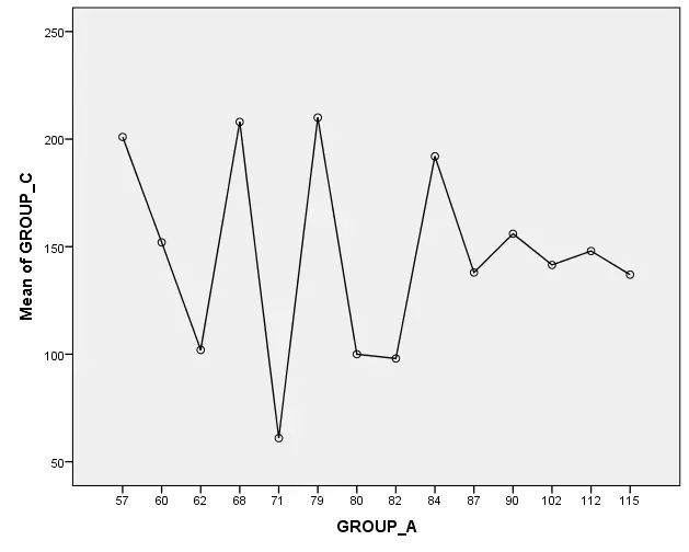
Figure 8: Mean plot of group c

Question 22

“Group B” is chosen as the level for the Y-axis of the bar graph.

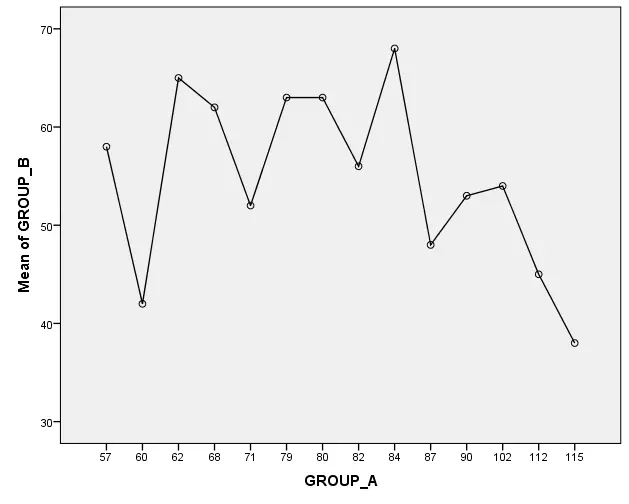
Figure 9: Mean plot of group B

Question 23

In presenting the bar chart within a scientific journal it is intended to look after Serum ferritin levels that were estimated in the three groups distinctly. The first group A proclaimed a fixed high-iron diet, the second group B maintained a low-iron diet and the last group estimated a control diet. In this analysis, the provided data is presented as the mean with some calculation with standard deviation (Love, et al. 2019). Also, notable differences are statistically denoted with asterisks. This figure transparently and briefly sustains that the provided data is introduced significantly. Also with the help of this chart, some noticeable considerations are evaluated that are described below.

This figure illustrates the visual understanding of the data and also summarizes the major results of the analysis. A brief illustration of the observed design including the observed groups, the considerations, and the number of the groups of each part is this figure. This figure also briefly explains the main findings of the statistical analysis and the outcomes of these tests (Baak, et al. 2020). Lastly, the code is also explained in a transparent and compact style which is essential for proper understanding for individuals who have not no need to read the whole analysis properly.

Figure 10: Anova test

Question 24

For interpreting the data the represented image here is the consideration of the outcomes from the one-way ANOVA test in the SPSS. The outcomes of the one-way ANOVA examination predicted that the three groups' serum ferritin levels varied statistically greatly (p < 0.05). This implies that the serum ferritin levels of the two groups are not identical for a minimum of one of the two classifications. To determine which group is diverse from the other groups, here is provided in the Anova tests various tables of comparisons, these tables illustrate the outcomes of all possible comparisons between the categories (Chatterjee, 2021). This multiple table also illustrated that the serum ferritin level in group c is notably increaser than the remaining two groups, so by understanding these results it can be said that group c is a group which consists of the minimum amount of diverse serum ferritin level rather comparing with the other two groups. This result also becomes more understanding when looking at the table of the direction of the difference. This implies that compared to the other two groups, Group C has a larger iron storage. It is a valuable indicator of iron level since it offers the general amount of iron held in the body as well as the quantity of iron that is general for the body to utilize. It is noteworthy to notice that Group C's larger iron storage than the other two groups cannot be explained by the one-way ANOVA test. Further investigation is required to ascertain the fundamental reason for this variation. A guy should consult his physician if he has concerns about his iron levels. To assess his serum ferritin level and other iron-related indicators, the doctor might prescribe a blood test (Shrestha, 2020). His doctor could suggest iron removal therapy, dietary modifications, or other therapies if his blood ferritin levels are elevated.

Scenario 4: The importance of study

Question 25

Pearson

Question 26

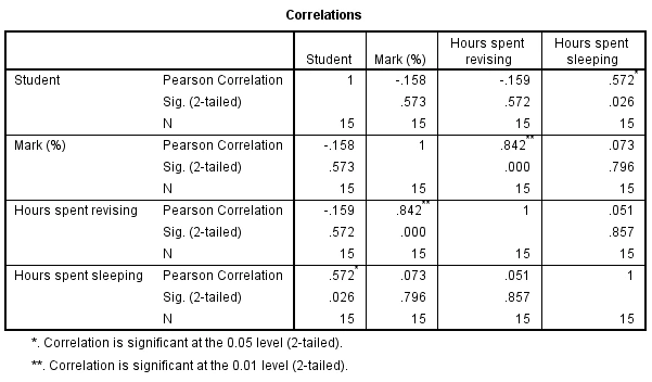
Figure 11: Pearson’s correlation

Since Pearson's correlation enables you to evaluate the linear connection between two continuous variables, that is why you choose it to examine the data in scenario 4. The data is made up of each student's continuous test scores and uninterrupted time spent studying and sleeping (Howitt, and Cramer, 2020). When determining the direction and degree of a relationship between two numerical variables, Pearson's correlation is the suitable statistical test to use. It satisfies the linearity and continuous paired data requirements. Correlations among continuous variables cannot be readily evaluated by other tests such as chi-squared, t-tests, or ANOVA. Pearson's rank correlation is more appropriate than Spearman's since the data seems to be fairly regularly distributed. In general, the most effective statistical technique to ascertain if test scores are associated with review or sleep duration is Pearson's correlation.

Question 27

Scatter plot

Question 28

Individual Data

Question 29

The title of the X axis is Hours Spent Revising

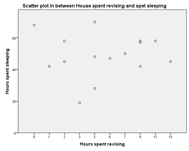
Figure 12: Scatter plot

Question 30

The title of the Y axis is Hours Spent Sleeping

Question 31

Pearson’s correlation

The exam score, hours spent reviewing, and hours spent sleeping for each of the 15 students are shown in this table based on the findings of Pearson's correlation tests.

Exam scores and sleep duration showed a strong positive connection (r=0.572, p=0.026). Test results tend to rise in correlation to sleep duration.

Test outcomes were significantly positively correlated with the amount of time put into studying (r=0.842, p<0.001). Higher exam scores were obtained by students who dedicated more time to revision (Huang, 2023).

There was no association between the order of students and their grades, according to the non-significant correlation between student (participant number) and exam mark (r=-0.158, p=0.573).

As a whole, the strong associations reveal that greater test performance is correlated with more sleep and revision time, however, there was no association found between student order and exam performance. The information is consistent with the theory that last-minute editing is detrimental.

Scatter plot

The graphic displays a scatter plot showing the correlation between the number of hours slept and the home where revisions are made. The amount of hours spent editing is shown by the x-axis, and the number of hours slept by the y-axis. A single point of information is represented by every circle on the scatter plot.

Those who spend more time reviewing also tend to sleep less, according to the statistics, which indicates an adverse relationship between the two factors (Gravetter, et al. 2021) This is probably because editing detracts away other things to do, including sleeping, by taking effort and time.

The scatter plot demonstrates the wide range of variance in the data as well. While some individuals who spend more time reviewing nevertheless manage to obtain a decent night's sleep, those who spend less time revising tend to sleep less. This implies that other variables, such as unique differences in sleep requirements and behaviors, may affect sleep.

Question 32

The findings of a correlational study analyzing the association between test scores, hours spent preparing, and hours slept for fifteen students are described in the paragraph. Pearson's correlation tests revealed a significant beneficial association between test scores and hours slept (r=0.572, p=0.026), indicating a possible relationship between more sleep and improved exam results. The number of preparation hours and test outcomes showed a substantial positive connection (r=0.842, p<0.001), suggesting that students who prepared more were able to get higher test scores. However, there was no correlation between test outcomes and student order (r=-0.158, p=0.573), indicating that the order of students did not affect performance (Howitt and Cramer, 2020).

The positive correlations indicating that better scores are predicted by greater revision time and sleep corroborate the theory that last-minute revisions adversely affect test performance. Students who revise more often tend to sleep less, as shown by the negative association between revision hours and sleep that is shown using a scatter plot. This is probably because editing takes time and energy that might otherwise be spent sleeping. Variability in the data, however, suggests that there are more variables at play, such as variations in normal sleep patterns.

Reference list

Journals

Amin, T.T., 2021. Inferential statistics. 2019 Accessed on 26th November.

Baak, M., Koopman, R., Snoek, H. and Klous, S., 2020. A new correlation coefficient between categorical, ordinal and interval variables with Pearson characteristics. Computational Statistics & Data Analysis, 152, p.107043.

Carrasco, J., García, S., Rueda, M.M., Das, S. and Herrera, F., 2020. Recent trends in the use of statistical tests for comparing swarm and evolutionary computing algorithms: Practical guidelines and a critical review. Swarm and Evolutionary Computation, 54, p.100665.

Chatterjee, S., 2021. A new coefficient of correlation. Journal of the American Statistical Association, 116(536), pp.2009-2022.

DeBono, A., 2021. Research methods and statistics for the social sciences.

Ferreira, D.F., 2019. SISVAR: A computer analysis system to fixed effects split-plot type designs: Sisvar. Brazilian Journal of Biometrics, 37(4), pp.529-535.

Gravetter, F.J., Wallnau, L.B., Forzano, L.A.B. and Witnauer, J.E., 2021. Essentials of statistics for the behavioral sciences.

Howitt, D. and Cramer, D., 2020. Understanding statistics in psychology with SPSS. Pearson.

Howitt, D. and Cramer, D., 2020. Understanding statistics in psychology with SPSS. Pearson.

Huang, H.N., 2023. Statistics reform: practitioner's perspective. Statistics.

Love, J., Selker, R., Marsman, M., Jamil, T., Dropmann, D., Verhagen, J., Ly, A., Gronau, Q.F., Šmíra, M., Epskamp, S. and Matzke, D., 2019. JASP: Graphical statistical software for common statistical designs. Journal of Statistical Software, 88, pp.1-17.

Makowski, D., Ben-Shachar, M.S., Patil, I. and Lüdecke, D., 2020. Methods and algorithms for correlation analysis in R. Journal of Open Source Software, 5(51), p.2306.

Pour‐Aboughadareh, A., Yousefian, M., Moradkhani, H., Poczai, P. and Siddique, K.H., 2019. STABILITYSOFT: A new online program to calculate parametric and non‐parametric stability statistics for crop traits. Applications in Plant Sciences, 7(1), p.e01211.

Shrestha, N., 2020. Detecting multicollinearity in regression analysis. American Journal of Applied Mathematics and Statistics, 8(2), pp.39-42.

Turhan, N.S., 2020. Karl Pearson's Chi-Square Tests. Educational Research and Reviews, 16(9), pp.575-580.